California Housing Price Prediction: A Comparative ML Workflow
Overview
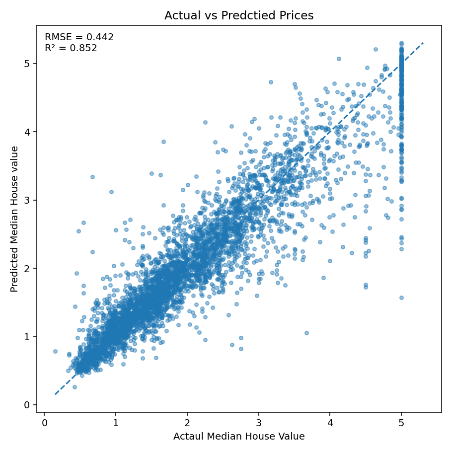
This project implements a rigorous, end-to-end machine learning workflow to predict median house values in California census block groups. The primary goal was to systematically compare the performance of diverse modeling techniques—from classical regression to advanced boosting(XGBoost, \(R^{2}\): 0.852 & RMSE: 0.442 ) and deep learning—while demonstrating proficiency in feature engineering, feature selection, and model optimization.
Tech Stack: Python, Scikit-Learn, NumPy, Pandas,
Matplotlib, Pytorch
Key Skills: Regression, Feature Engineering, Random
Forests, XGBoost, Deep Learning, Feature Importance
Links & Artifacts
Why this project
Tabular data problems are at the core of many real-world applications. This project demonstrates a complete, reproducible ML workflow — from baseline models to optimized ensemble learning and interpretability end-to-end, reproducible ML workflow: from baseline → iteration → validation → performance improvement → interpretation.
Comparative Results Summary
The iterative process led to a significant 28.6% reduction in prediction error (RMSE) compared to the initial Decision Tree model, with the XGBoost model achieving the best overall score.
| Model | Feature Count | RMSE | \(R^{2}\) Score | \(\Delta\) Improvement (RMSE Reduction) |
|---|---|---|---|---|
| Decision Tree (Baseline) | 11 | \(0.6096\) | \(0.7194\) | Baseline |
| Random Forest (Selected) | 7 | \(0.5020\) | \(0.8090\) | \(+17.7\%\) |
| XGBoost (Selected) | 7 | $ 0.4420 $ | \(0.8520\) | \(+27.5\%\) |
| XGBoost (with Clustering) | \(7 + 14\) | \(0.4355\) | \(0.8567\) | \(+28.6\%\) |
| PyTorch MLP Regressor | \(7 + 14\) | \(0.6630\) | \(0.6680\) | - |
Final Model Performance: The optimized XGBoost Regressor achieved a very high \(R^{2}\) score of \(\mathbf{0.8567}\), explaining over \(85\%\) of the variance in home prices.
Methodology and Optimization Pipeline
The project followed an iterative, three-phase approach, prioritizing performance gains and model efficiency:
1. Baseline and Initial Strategy
- Baseline Models: Standard Linear Regression and initial Decision Tree models established the performance floor.
- Initial Feature Engineering: An attempt to create
new, ratio-based features (e.g.,
bedrooms_per_room) was performed. This step was crucial as it demonstrated that the engineered features did not improve performance on tree models, leading to a pivot in strategy.
2. Strategic Feature Selection and Ensemble Learning
After observing diminishing returns from manual feature engineering, the focus shifted toward model-driven optimization through feature importance and ensemble learning.
- Feature Importance: A Decision Tree model was used to rank feature importance, leading to the elimination of low-impact variables. This strategic feature selection reduced the feature set from 11 to 7, resulting in a slight performance gain and a more efficient model.
- Ensemble Power (Random Forest): The optimized 7-feature set was used to train a Random Forest Regressor, which delivered the first major performance leap.
- Advanced Boosting (XGBoost): An XGBoost Regressor was applied with aggressive hyperparameter tuning. This boosting algorithm achieved the project’s highest accuracy on the initial feature set.
3. Advanced Feature Engineering & Deep Learning Benchmark
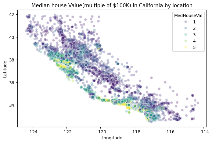
- Location Clustering (K-Means): Recognizing that
LatitudeandLongitudewere among the top predictors, K-Means Clustering was applied to the coordinates to create a new categorical region feature. Re-training the XGBoost model on this enhanced feature set delivered the final, best-performing result. - Deep Learning Benchmark (PyTorch MLP): A fully connected Multi-Layer Perceptron (MLP) was implemented in PyTorch to benchmark performance against tree-based ensembles. This step demonstrated proficiency with deep learning frameworks, data preparation for neural networks (scaling, custom data loaders), and benchmarking, even though the XGBoost model maintained superior performance.
Technical Stack and Takeaways
| Category | Tools & Techniques |
|---|---|
| Classical ML | Scikit-learn, Random Forest, XGBoost, Linear Regression, Decision Tree. |
| Feature Engineering | Feature Importance analysis, Feature Selection, K-Means Clustering for spatial feature creation. |
| Deep Learning | PyTorch (custom
Dataset, DataLoader, nn.Module
definition), \(\text{nn.MSELoss()}\),
\(\text{Adam}\) optimizer, GPU/MPS
device optimization. |
| Data & Metrics | Pandas, NumPy, RMSE, \(R^2\) Score. |
| Model Persistence | Final XGBoost model was saved using
joblib for deployment. |

What I learned
- Iterative Optimization: Demonstrated a principled approach by using initial models to guide later, more complex steps (Feature Importance over failed Feature Engineering).
- Handling Tabular Data: Confirmed that ensemble and boosting methods (XGBoost) are often superior to simple Deep Learning architectures for structured, tabular data.
- Cross-Platform Proficiency: Successfully implemented and benchmarked models in both the Scikit-learn/XGBoost ecosystem and the PyTorch deep learning framework, demonstrating versatility.
