Modeling Broadband Cloaking Using Nano-Assembled Plasmonic Meta-Structures
Imran Khan
Introduction & Motivation
Plasmonic cloaking suppresses the optical scattering signature of an object by engineering a shell whose induced response cancels the object’s far-field scattering. In the visible and near‑infrared regime, this relies on:
- Localized surface plasmon resonances (LSPRs)
- Phase-engineered destructive interference
- Strong multiple scattering within nanoparticle ensembles
A dielectric sphere exhibits Mie scattering, producing resonances based on refractive index contrast, core size, and wavelength. The goal of cloaking is to erase that optical fingerprint.
Why traditional cloaking models fail
Classical approaches such as Maxwell–Garnett effective medium theory fail for:
- dense, multilayer NP shells
- multiple scattering interactions
- large core sizes (d ∼ λ)
- size- and phase-dispersive AuNP optical responses
This work solves these limitations using a hybrid MFS + Foldy–Lax multiscale solver that accurately models:
- full-wave scattering from the core
- multiple scattering between hundreds to thousands of AuNPs
- shell–core interactions
- realistic material response
Physical Principles Behind Plasmonic Cloaking
Destructive Interference
Let the core and shell produces scattering, $ f_{core} $ and $f_{shell}$
Cloaking requires:
$$ f_{total} = f_{core} + f_{shell} \approx 0$$
This demands:
- Magnitude match — shell scattering must be
strong
- Phase opposition — induced polarization must be
anti-phase
- Broadband response — maintained over a spectral window
Why AuNP shells work
The extinction spectrum of AuNPs has a broad FWHM around 520 nm, enabling broadband cancellation between 400–600 nm. The strong scattering and absorption of the AuNPs creates intense local fields inside the shell, driving destructive interference with core scattering.
Computational methods:
This section briefly states the computational procedure for modeling scattering cross-section of a plasmonic meta-structures .
- Interaction of the monochromatic light with the dielectric core was computed using Methods of Fundamentals of Solutions(MFS).
- Multiple scattering and absorption by the nanoparticles in the shell and the core was computed using generalized Foldy-Lax scattering theory following a modification.
- Total scattered power by the meta-strucutre was computed using the Optical Theorem \(\sigma_{t}=\frac{4\pi}{k_{0}}Im[f(\hat{o},\hat{i})]\)
Modeling Assumptions:
- Metallic nanopparticles in the shell are assumed as point scatterer.
- A point scatterer has isotropic scattering pattern.
- Extinction properties of a point scatterer was attributed to a parameter, \(\alpha\), known as strength parameter as well. \(\alpha = [\frac{\sigma_{s}}{4\pi}-(\frac{k_{0}\sigma_{t}}{4\pi})]^{1/2} +\frac{ik_{0}\sigma_{t}}{4\pi}\)] where total cross-section of a point scatterer, \(\sigma_{t} = \sigma_{s}+\sigma_{a}\)
- The scattering (\(\sigma_{s}\)) and the absorption (\(\sigma_{a}\)) cross-sections were computed using Rayleigh Scatterig theory.
Problem statement and solution method
A plane wave with wavelength $\lambda$ propagates in the $+\hat{z}$ direction and is incident on a structure consisting of a dielectric sphere with radius \(a_{0}\) surrounded by \(N\) small, metal nanoparticles. The metal nanoparticles may be situated at subwavelength distances away from the surface of the dielectric sphere. Hence, the field scattered by this structure is the result of strong multiple scattering interactions between each and all of the components of the structure. In what follows, we describe a method to compute the field scattered by this structure. For simplicity, we describe the problem for scalar waves. In particular, we use the method of fundamental solutions(MFS) to compute scattering by the dielectric sphere and the Foldy-Lax equations to model the multiple scattering by the point particles that surround the sphere. Suppose that the origin of a coordinate system lies at the center of the dielectric sphere. We denote the interior domain by \(D = \{ r < a \}\) and the exterior domain by \(E = \{ r > a \}\). The spherical surface \(B = \{ r = a \}\) is interface between the interior and exterior. The wave field in the interior is denoted by \(\psi^{\text{int}}\) and satisfies the homogeneous reduced wave or Helmholtz equation,\[\left( \nabla^{2} + k_{1}^{2} \right) \psi^{\text{int}} = 0, \quad \text{in $D$}, \] with \(k_{1}\) denoting the wavenumber for the dielectric sphere. The wave field in the exterior is denoted by \(\psi^{\text{ext}}\) and satisfies \[ \left( \nabla^{2} + k_{0}^{2} \right) \psi^{\text{ext}} = -k_{0}^{2} \sum_{n = 1}^{N} V_{n} \psi^{\text{ext}}, \quad \text{in $E$}.\]
Here, \(k_{0}\) is the wavenumber for the exterior and \(V_{n}\) corresponds to the scattering potential for the \(n\)th metal nanoparticle. We write \(\psi^{\text{ext}}\) as the sum
$ \psi^{\text{ext}} = \psi^{\text{inc}} + \psi^{s}$
with \(\psi^{\text{inc}}\) denoting the incident field satisfying \[ \left( \nabla^{2} + k_{0}^{2} \right) \psi^{\text{inc}} = 0, \quad \text{in $R^{3}$},\]
and \(\psi^{\text{s}}\) denoting the scattered field satisfying \[ \left( \nabla^{2} + k_{0}^{2} \right) \psi^{\text{s}} = -k_{0}^{2} \sum_{n = 1}^{N} V_{n} \psi^{\text{inc}} - k_{0}^{2} \sum_{n = 1}^{N} V_{n} \psi^{\text{s}}, \quad \text{in $E$}. \]
We must supplement the equations above with conditions on \(B\) as well as radiation conditions. We prescribe that
\[ \psi^{\text{int}} = \psi^{\text{inc}} + \psi^{\text{s}} \quad \text{on $B$}, \] and \[ \partial_{\nu} \psi^{\text{int}} = \partial_{\nu} \psi^{\text{inc}} + \partial_{\nu} \psi^{\text{s}} \quad \text{on $B$}, \] with \(\partial_{\nu}\) denoting the derivative along the normal on \(B\) pointing into \(E\). Additionally, we require that \(\psi^{s}\) satisfies the Sommerfeld radiation condition. The differential equations supplemented by the interface conditions, and the requirement that \(\psi^{\text{s}}\) satisfies the Sommerfeld radiation condition constitute a complete mathematical description of the problem.
Interior field
To compute the interior field, we make use of the Method of Fundamental Solutions (MFS) which is also known as the Discrete Source Method. This method relies on knowing Green's function, denoted by \(G_{1}\), which satisfies \[ \left( \nabla^{2} + k_{1}^{2} \right) G_{1} = -\delta(r - r')\] the Sommerfeld radiation condition. It is given explicitly by \begin{equation} G_{1}(r - r') = \frac{e^{\mathrm{i} k_{1} | r - r '|}}{4 \pi | r - r' |}, \end{equation} which is a spherical wave centered at \(r'\) propagating in the whole space with wavenumber \(k_{1}\).
The key observation is that when \(r' \not\in D\), \(G_{1}\) exactly satisfies the differential equation for \(\psi^{\text{int}}\) since \(\delta(r - r') = 0\) for \(r \in D\) and \(r' \not\in D\). Because of this, we consider a set of \(M\) points \(r_{j}^{\text{int}} \in E\) for \(j = 1, \cdots, M\) and form the following approximation, $$\psi^{\text{int}}(r) \sum_{j =1}^{M} c^{\text{int}}_{j} G_{1}(r - \rho^{\text{int}}_{j}),r \in D. $$ This approximation is an exact solution of the differential equation for \(\psi^{\text{int}}\) for any set of points \(\rho_{j}^{\text{int}} \in E\) for \(j = 1, \cdots, M\). It is an approximation of the solution of this scattering problem because it does not exactly satisfy the boundary conditions. Rather, we will require that this approximation satisfies the boundary conditions only at a set of \(M\) points, which is called a collocation method.
In practice, we would like to have these points uniformly sample the interface \(B\) to make the approximation of the interface conditions as accurate as possible. Suppose the set of \(M\) points \(\rho^{\text{bdy}}_{j} \in B\) for \(j = 1, \cdots, B\) uniformly sample (or close to uniformly sample) the sphere of radius \(a_{0}\). Then, we set $$\rho^{\text{int}}_{j} = \rho^{\text{bdy}}_{j} + \ell \nu_{j}, \quad j = 1, \cdots, M, $$ with \(\nu_{j}\) denoting the unit outward normal at \(r_{j}\), and \(\ell > 0\) denoting a user-defined length parameter which we typically set to be smaller than a wavelength.
Exterior field
To approximate \(\psi^{\text{ext}}\) we make use of Green's identity which essentially states that the exterior field is given by a superposition of surface and volume sources. Here, surface sources correspond to scattering by the dielectric sphere and volume sources correspond to the \(N\) metal nanoparticles. In what follows, we approximate the surface sources using the Method of Fundamental Solutions and the volume sources using the self-consistent Foldy-Lax scattering theory, which is a scalar wave theory closely related to what is used in the Discrete Dipole Approximation.
In what follows, we represent \(\psi^{\text{ext}}\) as the following sum, \[\psi^{\text{ext}} = \psi^{\text{inc}} + \underbrace{\psi^{B} + \sum_{n = 1}^{N} \Psi_{n}}_{\psi^{\text{s}}}, \] with \(\psi^{B}\) denoting the "surface source" field scattered by the dielectric sphere and \(\Psi_{n}\) denoting the "volume source" field scattered by the \(n\)th metal nanoparticle. We describe our approximations for each of these scattered fields below.
Field scattered by the dielectric sphere
We use the Method of Fundamental solutions to compute the field
scattered by the dielectric sphere. Here, we use the Green's function
\(G_{0}\) satisfying $$ \left(
\nabla^{2} + k_{0}^{2} \right) G_{0} = -\delta(r - r'), $$ and the
Sommerfeld radiation condition, which is given explicitly by \[
G_{0}(r - r') = \frac{e^{\mathrm{i} k_{0} | r - r' |}}{4 \pi |
r -
r' |}.\] Just as we have done for the interior field, we
introduce the set of M points,
\[\rho_{j}^{\text{ext}} = \rho^{\text{bdy}}_{j} -
\ell \nu_{j},\quad j = 1, \cdots, M. \]
Field scattered by the metal nanoparticles
Let us denote the center of the \(n\)th metal nanoparticle by \(R_{n}\). In what follows, we assume that each of the \(N\) metal nanoparticles is small enough that we can account for its scattering properties by a scattering coefficient, \(\alpha_{n}\), which may depend on \(\lambda\). It follows that the field scattered by the \(n\)th metal nanoparticle is given by \[ \Psi_{n}(r) = \alpha_{n} G_{0}(r - R_{n}) \Psi_{E}(R_{n}),\] with \(G_{0}\) denoting the Green's function defined above and \(\Psi_{E}(R_{n})\) denoting the exciting field evaluated at \(R_{n}\). Supposing that \(R_{n}\) and \(\alpha_{n}\) for \(n = 1, \cdots, N\) are known, all that remains to be determined is \(\Psi_{E}(R_{n})\) for \(n = 1, \cdots, N\).
To determine this exciting field, we use Foldy-Lax theory which we describe below. Foldy-Lax theory is a self-consistent multiple scattering theory. It is not an exact theory, but it does account for infinitely many interactions between the metal nanoparticles, so it provides a useful multiple scattering model. This theory is limited to settings in which the metal nanoparticles are not too densely distributed over the dielectric sphere so that these scattering elements are statistically independent.
We model the field exciting the \(n\)th metal nanoparticle as the following sum, \[ \Psi_{E}(R_{n}) = \psi^{\text{inc}}(R_{n}) + \psi^{B}(R_{n}) + \sum_{\substack{n' = 1\\ n' \neq n}}^{N} \sigma_{n'} G_{0}(R_{n} - R_{n'}) \Psi_{E}(R_{n'}). \] This equation gives the exciting field at \(r_{n}\) as the sum of the incident field \(\psi^{\text{inc}}\), the field scattered by the dielectric sphere \(\psi^{B}\), and the fields scattered by all of the other \(N-1\) metal nanoparticles evaluated at \(r_{n}\). By rearranging this equation and considering it for each and all \(N\) metal nanoparticles, we obtain the \(N \times N\) linear system, \[ \Psi_{E}(R_{n}) - \sum_{\substack{n' = 1\\ n' \neq n}}^{N} \sigma_{n'} G_{0}(R_{n} - R_{n'}) \Psi_{E}(R_{n'}) = \psi^{\text{inc}}(R_{n}) + \psi^{B}(R_{n}), \quad n = 1, \cdots, N. \] Upon solution of this linear system, we obtain \(\Psi_{E}(r_{n})\) for \(n = 1, \cdots, N\). This result can then be used to evaluate \[ \Psi(r) = \sum_{n = 1}^{N} \alpha_{n} G_{0}(r - R_{n}) \Psi_{E}(R_{n}), \quad r \in E. \] This field gives the field scattered by the entire set of \(N\) metal nanoparticles. Because this field is given as a superposition of Green's functions, each of which satisfies the Sommerfeld radiation condition, it follows that \(\Psi\) satisfies the Sommerfeld radiation condition.
Interface conditions
At this point we have introduced approximations for the interior and exterior fields. Both are exact solutions of the associated differential equations and the exterior field satisfies the Sommerfeld radiation condition. All that remains is to require that these fields satisfy interface conditions given in Section 1.
Let us review what we have so far. The approximation of the interior field is given by \[ \psi^{\text{int}}(r) \cong \sum_{j = 0}^{M} c_{j}^{\text{int}} G_{1}(r - \rho_{j}^{\text{int}}) \quad r \in D. \] The approximation of the exterior field is given by \[ \psi^{\text{ext}}(r) \cong \psi^{\text{inc}}(r) + \underbrace{\sum_{j = 1}^{M} c_{j}^{\text{ext}} G_{0}(r - \rho_{j}^{\text{ext}})}_{\psi^{B}} + \sum_{n = 1}^{N} \alpha_{n} G_{0}(r - R_{n}) \Psi_{E}(R_{n}), \quad r \in E,\] with \(\Psi_{E}(R_{n})\) satisfying \[ \Psi_{E}(R_{n}) - \sum_{\substack{n' = 1\\ n' \neq n}}^{N} \sigma_{n'} G_{0}(R_{n} - R_{n'}) \Psi_{E}(R_{n'}) \] \[ = \psi^{\text{inc}}(R_{n}) + \sum_{j = 1}^{M} c_{j}^{\text{ext}} G_{0}(R_{n} - \rho_{j}^{\text{ext}}), \quad n = 1, \cdots, N. \] The quantities \(c_{j}^{\text{int}}\) for \(j = 1, \cdots, N\), \(c_{j}^{\text{ext}}\) for \(j = 1, \cdots, N\), and \(\Psi_{E}(R_{n})\) for \(n = 1, \cdots, N\) are to be determined.
By requiring that the interface condition for the fields is satisfied exactly on the \(M\) boundary points, \(\rho^{\text{bdy}}_{i} \in B\) for \(i = 1, \cdots, M\), we find that
\[ \sum_{j = 0}^{M} c_{j}^{\text{int}} G_{1}(\rho^{\text{bdy}}_{i} - \rho_{j}^{\text{int}}) - \sum_{j = 1}^{M} c_{j}^{\text{ext}} G_{0}(\rho^{\text{bdy}}_{i} - \rho_{j}^{\text{ext}}) - \sum_{n = 1}^{N} \alpha_{n} \] \[ G_{0}(\rho^{\text{bdy}}_{i} - R_{n}) \Psi_{E}(R_{n}) = \psi^{\text{inc}}(\rho^{\text{bdy}}_{i}),\quad i = 1,\cdots, M. \]
Similarly, by requiring that the interface condition for the normal derivatives of the fields is satisfied exactly on the \(M\) boundary points, we find that\[\sum_{j = 0}^{M} c_{j}^{\text{int}} \partial_{\nu} \\ G_{1}(\rho^{\text{bdy}}_{i} - \rho_{j}^{\text{int}}) - \sum_{j = 1}^{M} c_{j}^{\text{ext}} \partial_{\nu} G_{0}(\rho^{\text{bdy}}_{i} - \rho_{j}^{\text{ext}})\] \[-\sum_{n = 1}^{N} \alpha_{n} \partial_{\nu} G_{0}(\rho^{\text{bdy}}_{i} - R_{n}) \Psi_{E}(R_{n})=\partial_{\nu} \psi^{\text{inc}}(\rho^{\text{bdy}}_{i}), \quad i = 1, \cdots, M.\]
Finally, by rearranging terms in this equation, we find that \[ \Psi_{E}(R_{n}) - \sum_{\substack{n' = 1\\ n' \neq n}}^{N} \alpha_{n'} G_{0}(R_{n} - R_{n'}) \Psi_{E}(R_{n'}) \] \[- \sum_{j = 1}^{M} c_{j}^{\text{ext}} G_{0}(R_{n} - \rho_{j}^{\text{ext}})= \psi^{\text{inc}}(R_{n}) , \quad n = 1, \cdots, N.\] These three equations give \(2MN\) equations for the \(2MN\) unknowns, \(c_{j}^{\text{int}}\) for \(j = 1, \cdots, M\), \(c_{j}^{\text{ext}}\) for \(j = 1, \cdots, M\), and \(\Psi_{E}(r_{n})\) for \(n = 1, \cdots, N\). These equations can be combined to form a \(2MN \times 2MN\) linear system that can be solves using standard numerical linear algebra methods.We now present the codes that computes the solution of this linear system and uses that result to compute the field scattered by this cloaking structure.
Computing the total scattering cross-section
After solving the system of linear equation described in the last section (avobe), thescattered filed is given by,
\[\psi^{s}(r) = \psi^{B} + \sum_{n=1}^{N} \Psi_{n}\approx \sum_{j=1}^{M}c_{j}^{ext}G_{0}(r-r_{j}^{ext}) + \sum_{n=1}^{N}\alpha_{n}G_{0} (r-r^{NP}_{n})\Psi_{E}(r_{n}^{NP}), r \in E.\]
The scattered field evaluated at \(\textbf{r}= R\hat{o}\) with \(R=|r|\) and \(\hat{o} = \textbf{r} / |\textbf{r}|\) in the far-field corresponding to \(R>>1\) behaves like a spherical wave and is given by,
\[\psi^{s} \sim f(\hat{o},\hat{i}) \frac{e^{ik_{0}}R}{R} \]
Here, \(f(\hat{o},\hat{i})\) is the scattering amplitude for the scattered field in the far field in the direction \(\hat{o}\) when the particle is illuminated by a plane wave propagating in the direction \(\hat{i}\) with unit amplitude.
Suppose we have set \(\psi^{inc}\) to be a plane wave of unit amplitude propagating in the direction \(\hat{i}\) and we have used that compute the the solution of the last three equation described in the section above. Using \(|R\hat{o}-r^{'}|\sim R- \hat{o}.r^{'}\) for \(R>>1\), in the far-field Green's function is ,
\[G_{0}(R\hat{o}-r^{'}) \sim e^{ik_{0}\hat{o}.r^{'}}\frac{e^{ik_{0}R}}{4\pi R}, R>>1\]
Replacing \(G_{0}\) by the first two equations from this section we get,
\[\psi^{s}(r) \sim \left[ \frac{1}{4\pi} \sum_{j=1}^{M} c_{j}^{ext} e^{ik_{0}\hat{o}.r^{ext}_{j}} + \sum_{n=1}^{N} \alpha_n e^{ik_{0}\hat{o}.r^{NP}_{n}} \Psi_{E}(r_{n}^{NP}) \right]\frac{e^{ik_{0}R}}{R}, R>>1\]
By comparing this last equation with the second equation from beginning of this section we find the scattering amplitude using our method given as,
\[f(\hat{o}, \hat{i}) = \frac{1}{4\pi} \sum_{j=1}^{M} c_{j}^{ext} e^{ik_{0}\hat{o}.r^{ext}_{j}} + \frac{1}{4\pi} \sum_{n=1}^{N} \alpha_n e^{ik_{0}\hat{o}.r^{NP}_{n}} \Psi_{E}(r_{n}^{NP}) \]
According to the Optical Theorem of the forward scattering theorem, we can compute the total cross-section of the scattering structure through evaluation of ,
\[\sigma_{t} = \frac{4\pi}{k_{0}}Im[f(\hat{i},\hat{i})]\]
Now we can compute the total cross-section by substituiting equation above the last equation into this formula. Remarkably, the last equation of this section allows for the determination of \(\sigma_{t}\) by only measuring scattered power in the forward direction.
Computational challenges
- Matrix of size ( N imes N )
- Dense, non‑diagonal
- O(N³) cost with Gaussian elimination
Hybrid System Assembly
The final linear system includes:
- M boundary equations (continuity)
- M derivative boundary equations
- N Foldy–Lax equations
Matrix size:
(2M + N) X (2M + N)
Experimental Comparison
Matching the work of Mühlig et al. (Sci. Rep. 2013):
- Maxwell–Garnett predicts incorrect spectral position
- This model captures correct suppression between 340–390 nm
Results & Discussion
Scattering Efficiency of Core vs Core-Shell
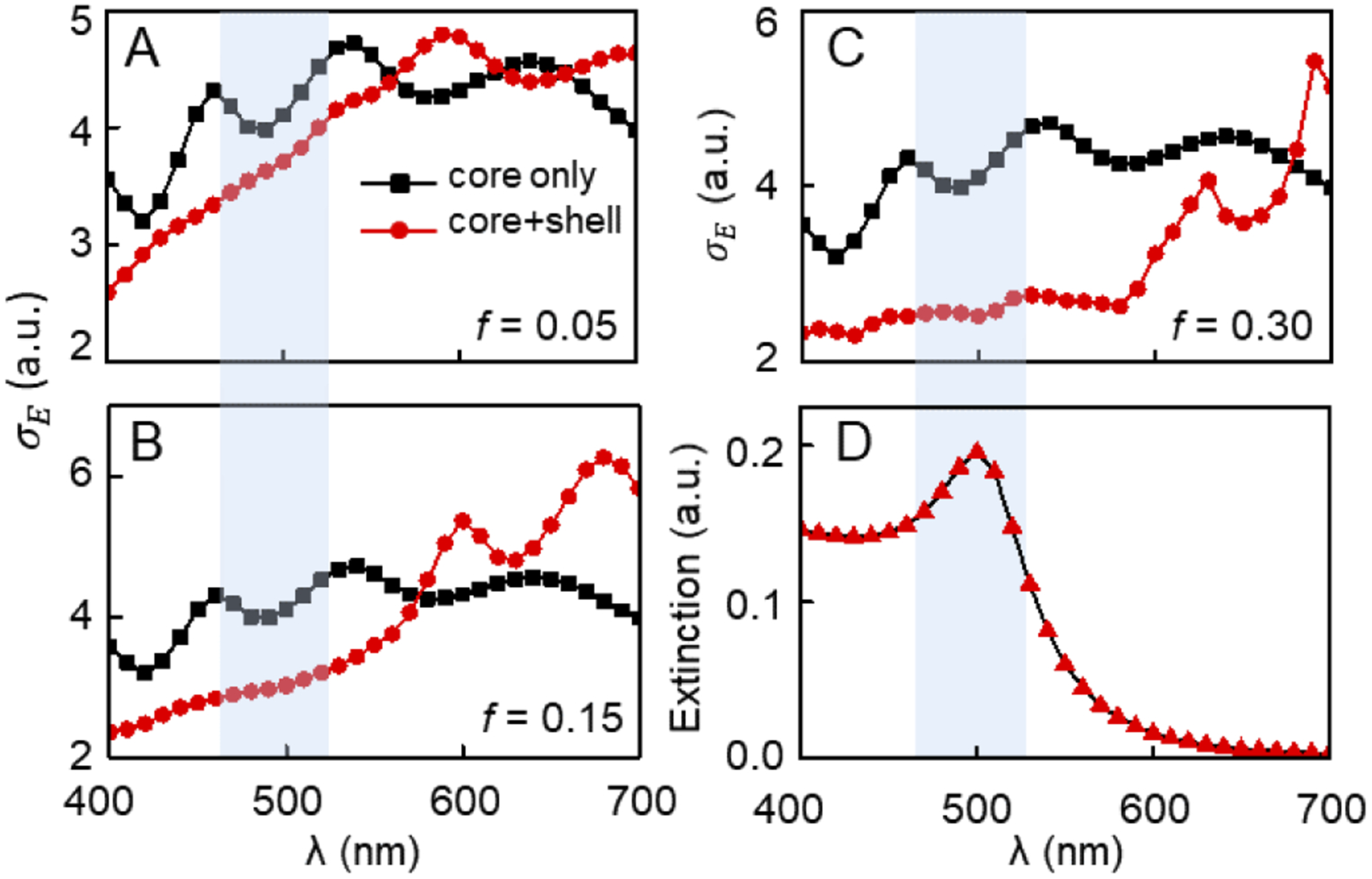
- Shell removes core’s Mie resonances
- Suppression overlaps with AuNP extinction FWHM
Effect of NP Size
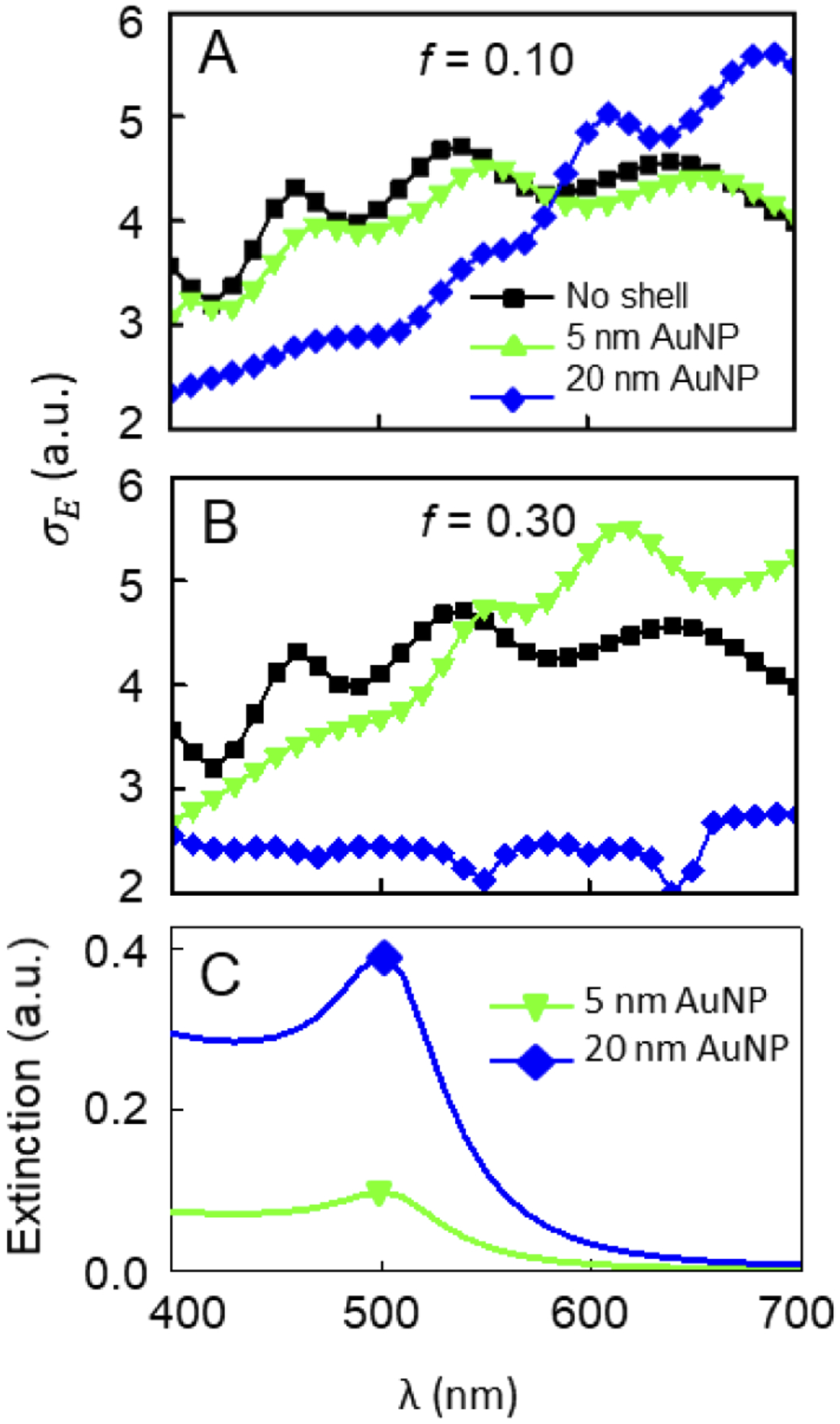
Larger AuNPs:
- exhibit stronger plasmonic response
- increase both absorption and scattering
- deliver deeper suppression
Filling Fraction Dependence
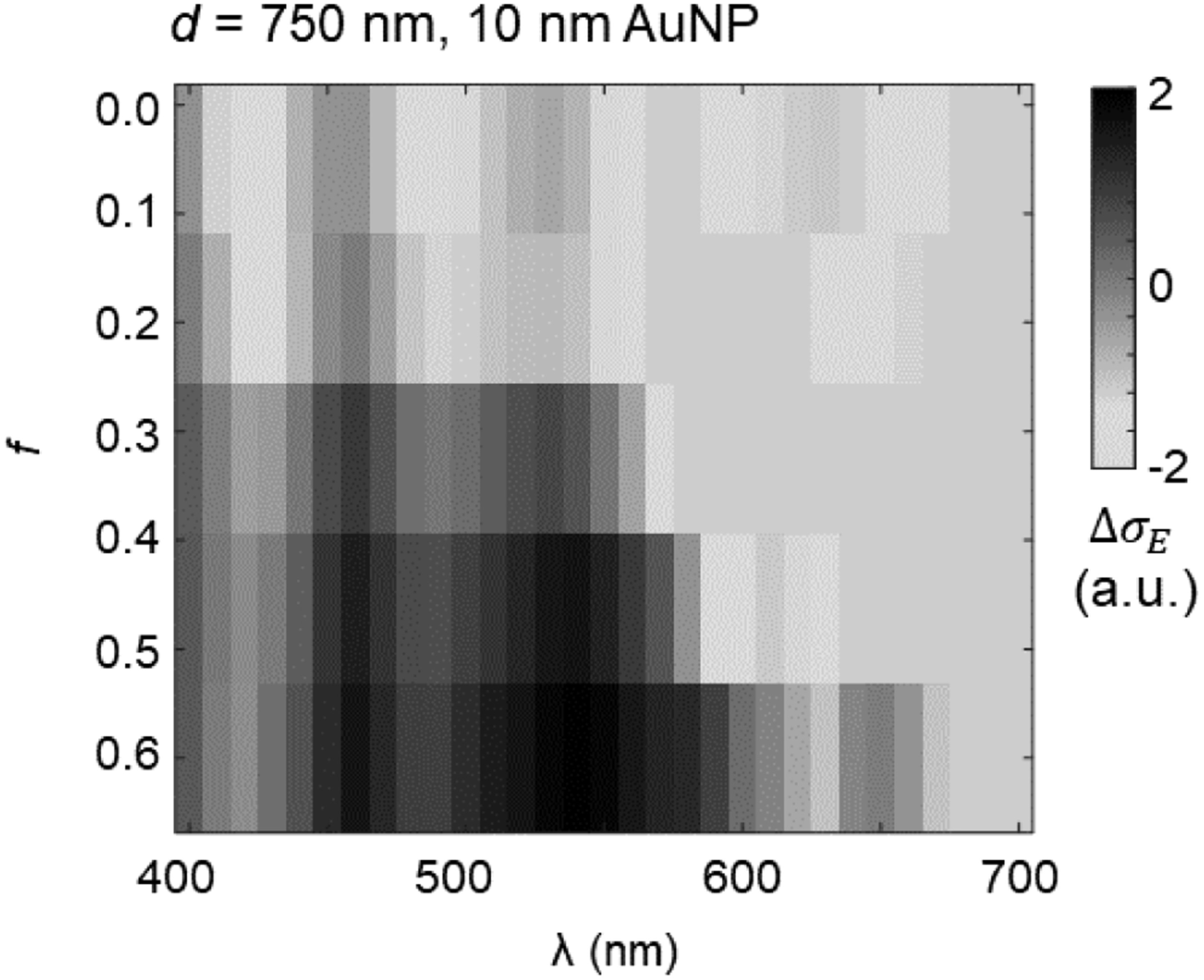
- Cloaking begins at f ≈ 0.25
- Increasing f broadens and deepens suppression
Scaling to Larger Cores
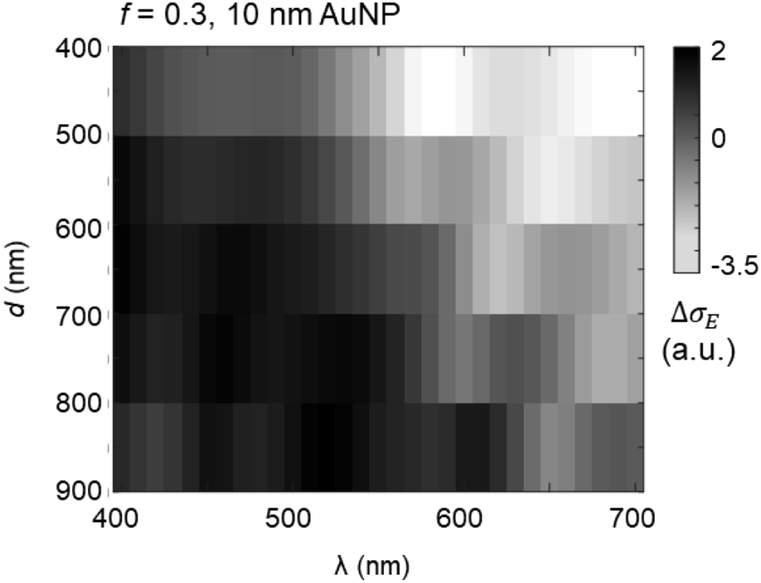
Even for shells around 900 nm cores, suppression remains strong without increasing shell layers.
Mechanistic Interpretation
Multiple Scattering Trap
Dense AuNP layers create:
- high local field intensities
- repeated scattering loops
- strong absorption channels
Anti-Phase Resonant Response
Shell-induced polarization cancels the core’s multipole radiation.
Extinction Bandwidth Determines Cloaking Band
Cloaking spectral range is governed by:
$\sigma_{\mathrm{ext}}(\lambda)$
of a single AuNP.
Limitations and Future Extensions
Current limitations
- Scalar approximation
- Point‑scatterer assumption
- No NP–NP near-field tunneling
- O(N³) computational complexity
Future improvements
- Vector MFS
- Fast multipole acceleration (FMM)
- GPU‑accelerated iterative solvers
- Polydisperse NP modeling
Applications Across Fields
Optics & Photonics
- cloaking
- metasurfaces
- nanoantenna scattering design
Semiconductor Metrology
- CD‑SEM scattering models
- contamination detection
- forward models for inverse imaging
Computer Vision & AI
- physics-informed ML
- imaging simulations for training pipelines
- advanced scattering-based augmentation
- explainable AI using wave models
Summary
This full technical deep dive captures:
- the physics of plasmonic cloaking
- complete derivation of the hybrid solver
- numerical engineering details
- validation against theory & experiment
- broadband cloaking demonstration
- scalability to large microspheres